Internal:GPCD

Introduction

Protein Cavities

Cavities are structural features of proteins and they are often important for drug discovery and design. There are different kinds of cavities, including pockets, voids, tunnels, and channels. The types of cavities are listed in more detail in figure 1.

Figure 1: The basic types of protein cavities [1]

1. Void: A cavity that looks like internal "hole" in a protein with no connection to the surface.
2. Cleft: A pocket that looks like a "dent" in the surface of a protein. Can also be found as part of a tunnel or channel.
3. Invagination: A pocket that looks like a "cove". It has a small opening on the surface of a protein and leads to a larger interior. Can also be found as part of a tunnel or after a cleft.
4. Tunnel: A pocket that has an opening on the surface of a protein and leads to somewhere in the interior. Has no opening on the other side.
5. Channel: A cavity that has an opening on one side of the surface of a protein and leads to another opening in another location on the surface of the protein.

Of course, the types of cavities listed in figure 1 are only the basic ones. Combinations of these are also possible as shown in figure 2.

Figure 2: Combination types of protein cavities [1]

Protein Cavity Detection Methods

There are several methods for detecting protein cavities. There are sphere based methods, grid based methods, grid-and-sphere based methods, surface based methods, grid-and-surface based methods, time-varying methods, GPU based methods, consensus based methods, and finally tessellation based methods. These algorithms are shown in more detail in figure 3. Tessellation based methods mainly rely on Voronoi tessellation. Some methods rely on weighted Voronoi tessellation because of its ability to more accurately represent the volume of atoms. The Voronoi tessellation in these methods is computed from a set of points representing the atomic centers of the underlying protein.

Figure 3: A hierarchy of protein cavity detection algorithms [1]

Literature Review

MOLE

Method

The MOLE algorithm is specifically designed to identify tunnels and channels. Finding superficial cavities is a secondary concern and does so as part of the surface approximation step. MOLE utilizes the surface obtained by the refinement of the convex hull to find superficial cavities such as clefts and invaginations. In essence, the approximation of a more accurate surface and the detection of these superficial cavities are closely related. As tetrahedra are removed from the convex hull to get a more accurate surface approximation, a parameter called interior threshold controls how many superficial cavities are found. For example, if the number of tetrahedra removed from a specific part of the molecule exceeds this threshold, the algorithm marks these tetrahedra as part of a superficial cavity.

Figure 4: Shows in 2D the Voronoi diagram (thin lines) and the convex hull (dotted line) of molecule represented by atoms (circles). Each Voronoi edge is evaluated by the cost function (numbers). The thick line represents the optimal path found by the Dijkstra's algorithm from the given starting point (black circle), i.e., centerline of found tunnel. [1]

For the more complicated types of cavities, tunnels and channels, MOLE uses the Voronoi diagram to identify them. Start and end points are defined as the centers of the deepest tetrahedra in each cavity. The depth of the tetrahedron is defined as the number of Voronoi edges from the closest boundary tetrahedron (on the surface). Tunnels/channels are computed as the shortest paths between all pairs of start and end points in the same cavity diagram.

Figure 5: Shows the weight function used to estimate the weight of each Voronoi edge for Dijkstra's algorihtm. l(e) is the length of the edge, d(e) is the distance of the edge to the closest atom Van der Waals sphere and ϵ is a small number to avoid division by zero [1]

Complexity

• Worst-case: O(N^2 log N), where N is the number of atoms in the molecule.
• Average: O(M log M), where M is the number of vertices in the Voronoi diagram (in the worst case, M = N^2, but in most cases M = O(N)). As a result of the use of the incremental algorithm and Hilbert curve ordering, the complexity of calculating the Delaunay triangulation of most molecular structures is O(N log N). Finally, the complexity of all the remaining steps of the algorithm is at most O(M log M).

MolAxis

Method

The MolAxis algorithm relies on Voronoi and Dijkstra's algorithm to find channels, similarly to MOLE. The algorithm consists of the following high-level steps:

1. Approximate the molecule using a collection of fixed-size spheres. The number of balls needed depends on the required quality of the approximation. In the extreme case, where the user is interested in a high resolution, each atom is approximated using a single sphere.
2. Compute the Voronoi diagram of the centers of the fixed-sized spheres. The diagram is intersected with a user-defined bounding sphere. This defines the area of interest.
3. Discard the parts of the Voronoi diagram that intersect the molecule.
4. Define a graph, using the Voronoi vertices and edges. A weight is given to each edge, which depends on its length and on its distance from the surface of the molecule.
5. Define a source point (root vertex). The user can either supply a source point or allow MolAxis to automatically choose the source point to be the center of the largest cavity in the molecule (basically detect channels inside-out).
6. Apply a shortest path optimization algorithm (Dijktra's algorithm) on the graph, computing a tree called the "corridor tree".
7. The desired channels are paths in the corridor tree. Duplicate channels are avoided by using the split distance parameter. The split distance bounds the distance to the least common ancestor of the channel and all previously reported channels.

Figure 6: Shows an example of fixed-size circles (light-blue) approximating varying-size circles and the pathway diagram of their centers. The discarded portion of the Voronoi diagram of their centers is depicted using dotted lines [2]. This figure also helps illustrate the usefulness of the Voronoi tessellation in computing pathways.

Possible Methods that need to be Explored

1. PODM Tessellation Using Van der Waals Surface Image (Angelos)

The first method that could be used for detecting protein cavities in parallel involves using PODM to create a tessellation of an image representation of the Van der Waals surface of a protein. The Van der Waals surface is an accurate representation of the surface of a protein and represents each atom as a sphere of a radius corresponding to its Van der Waals radius.

The steps for this method are outlined below:

1. Compute the Van der Waals surface (Angelos): This polygonal surface can be computed using UCSF Chimera. The output from this is an STL file containing the polygonal surface mesh. However, because the implementation is sequential, this step can present a major bottleneck in the overall method. In order to speed the process up, a custom parallel implementation to generate this surface will be necessary in the future.
2. Generate image of the Van der Waals surface (Angelos): Because PODM requires an image as input, the polygonal Van der Waals surface needs to be converted to an image. This is done by "filling" the polygonal surface with a constant value. The segmentation module of 3D Slicer can be used for doing this, but as before, this step can present a major bottleneck because the implementation is sequential. A custom parallel implementation is once again necessary.
3. Compute Delaunay tessellation using PODM: Once we have the image of the Van der Waals surface, we use PODM to compute the Delaunay tessellation in parallel. A low enough delta should be used to ensure that the surface is as accurately captured as possible.
4. Compute Voronoi tessellation using PODM: The next step is to compute the Voronoi tessellation as the dual of the Delaunay tessellation in parallel. The Voronoi tessellation is useful for quickly identifying tunnels using Dijkstra's algorithm.
5. Identify cavities in parallel (Angelos & Spiros): With the Delaunay and Voronoi tessellations computed, the cavities now need to be identified in parallel. It is crucial that this step is done in parallel as no other method implements "proper" parallelization. This is by far the most challenging step.
6. Output detected cavities as tessellations: The last step is to output the detected cavities as a tessellated mesh. It is important to only include the identified cavities in this mesh by representing them as tetrahedra. This way, researchers can overlay the normal protein structure with the tessellations of the cavities and easily see where they are.

• 
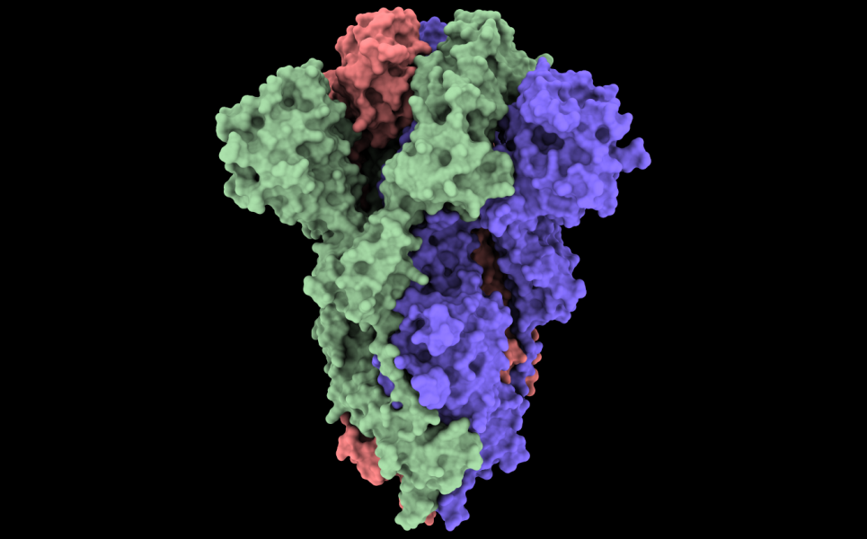  Figure 7: The Van der Waals surface of the COVID-19 spike glycoprotein (6vxx).
• 
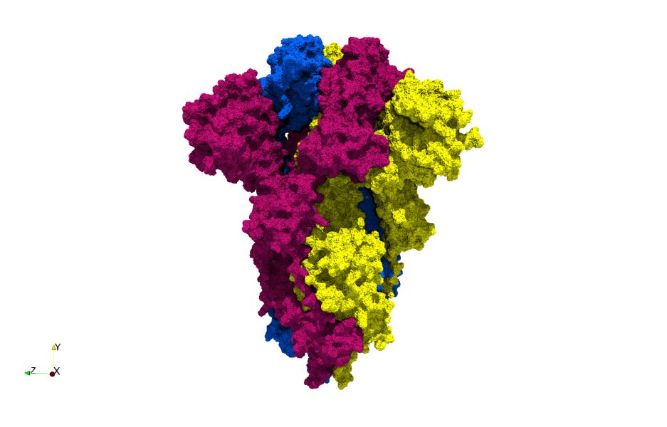  Figure 8: A tessellation based on the Van der Waals surface of the COVID-19 spike glycoprotein (6vxx). A highly-accurate surface tessellation is produced.

2. PDT Tessellation Using Point Cloud of Atoms (Spiros)

The second method involves giving PDT/PODM a point cloud of atoms and creating a tessellation from that. This would require that the Delaunay triangulation is generated and a method for computing an accurate surface for the point cloud is employed. Computing this surface is one of the most challenging steps of this method. A method that could be employed is α-shapes, but this has the disadvantage of not guaranteeing connectivity between tetrahedra. Another method probably needs to be used that can guarantee connectivity between the tetrahedra (such as the one from MOLE 2.5).

The steps for this method are outlined below:

1. Read PDB file and make point cloud of atoms (Angelos): The first step would be to read an input PDB file for a protein and create a point cloud of atoms. This involves either writing a basic PDB file reader or finding one we can use. However, writing a basic one is better because it skips the overhead of other full-featured readers as we only care about the atomic centers and potentially the type of atoms.
2. Compute Delaunay triangulation using PDT/PODM: The second step is to compute the Delaunay triangulation from the point cloud in parallel. This will produce an inaccurate surface that needs to be refined.
3. Compute accurate surface (Spiros): The Delaunay triangulation on a point cloud of atoms produces a surface that does not reflect the actual surface of the protein. As a result, an accurate surface needs to computed by refining the triangulation. This would involve removing tetrahedra until an accurate surface is found. This should be done in parallel.
   1. MOLE method:
      1. The molecular surface is approximated by iterative removal of boundary tetrahedra from the outermost layers (i.e., tetrahedra found at the interface between the molecule and the external environment).
      2. Boundary tetrahedra produced by the triangulation are removed in this step if they are sufficiently large to fit a sphere with a given probe radius
         1. Note: A tetrahedron T fits a sphere S with probe radius r if the center C of sphere S can be placed inside the tetrahedron and the distance to all vertices of T is greater than or equal to the sum of r, with the Van der Waals radius of an atom corresponding to the given vertex.
            1. Explanation: Given a boundary tetrahedron, if a Sphere S with center = Incenter C, and radius = probe radius
      3. Next, tetrahedra that are too small to fit a sphere with interior radius are removed.
         1. Explanation: Given a non-boundary tetrahedron, if the radius of its inscribed sphere is smaller than (probe?) radius, then the tetrahedron needs to be removed.
      4. Remaining tetrahedra form one or more connected components. We call the components that contain at least one tetrahedron on the molecular surface cavity diagrams.
      5. It should be noted here that the cavity diagram is a purely geometrical concept to help identify regions of space (volume) that can contain tunnels and only very loosely corresponds to the cavities shown in Figure 1B).
4. Compute Voronoi tesselation: Once the accurate surface is determined the Voronoi tessellation must be computed. This step could be done before the accurate surface is computed, but we would also have to refine the Voronoi if that is to happen.
5. Identify cavities in parallel (Angelos & Spiros): With the Delaunay and Voronoi tessellations computed, the cavities now need to be identified in parallel. It is crucial that this step is done in parallel as no other method implements "proper" parallelization. This is by far the most challenging step.
6. Output detected cavities as tessellations: The last step is to output the detected cavities as a tessellated mesh. It is important to only include the identified cavities in this mesh by representing them as tetrahedra. This way, researchers can overlay the normal protein structure with the tessellations of the cavities and easily see where they are.

• 
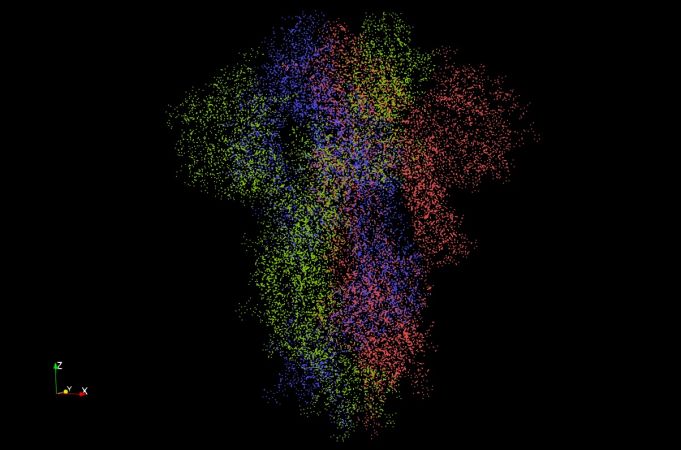  Figure 9: The atomic point cloud of the COVID-19 spike glycoprotein (6vxx). There are 23,694 atoms (points) in this image.
• 
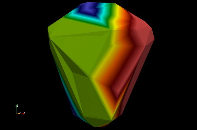  Figure 10: An unrefined Delaunay triangulation of the COVID-19 spike glycoprotein (6vxx). Generated using the Delaunay3D filter in ParaView.
• 
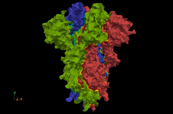  Figure 11: A Delaunay triangulation using α-shapes with α=3 of the COVID-19 spike glycoprotein (6vxx). Using α-shapes we can get a better approximation of the surface. Generated using the Delaunay3D filter in ParaView.

3. Surface-Grid-based Using Van der Waals Surface Volumetric Image

The third method involves writing a new software for doing protein cavity detection. This software would use a volumetric image (e.g. of type .mha) representing the Van der Waals surface of a protein. Uses perhaps the most faithful representation of the Van der Waals surface, which is the ground truth for a molecular surface. As long as the Van der Waal surface generation algorithm is fast, this method has the potential of being both accurate and fast as it eliminates the overhead of tessellation. Good parallelization is important for this method because there are many more voxels than there are tetrahedra in a tessellation-based method. Because this method operates on voxels, it is a candidate for future GPU parallelization. This method is also a strong candidate for deep learning, much more than the tessellation based methods, because its output can easily be used for training a deep learning model in the future.

The steps for this method are outline below:

1. Compute the Van der Waals surface: This polygonal surface can be computed using UCSF Chimera. The output from this is an STL file containing the polygonal surface mesh. However, because the implementation is sequential, this step can present a major bottleneck in the overall method. In order to speed the process up, a custom parallel implementation to generate this surface will be necessary in the future.
2. Generate image of the Van der Waals surface: Because PODM requires an image as input, the polygonal Van der Waals surface needs to be converted to an image. This is done by "filling" the polygonal surface with a constant value. The segmentation module of 3D Slicer can be used for doing this, but as before, this step can present a major bottleneck because the implementation is sequential. A custom parallel implementation is once again likely necessary in the future.
3. Identify cavities in parallel: Using the image voxels, the cavities now need to be identified in parallel (potentially using GPU parallelization in the future). It is crucial that this step is done in parallel as no other method implements "proper" parallelization. This is by far the most challenging step.
4. Output detected cavities as volumetric image: The last step is to output the detected cavities as a volumetric important. It is important to only include the identified cavities in this image. This way, researchers can overlay the normal protein structure with the volume of the cavities and easily see where they are.

• 
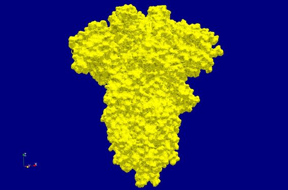  Figure 12: Volumetric image of the Van der Waals surface of the COVID-19 spike glycoprotein (6vxx). There are 15.5 million voxels in this volume.
• 
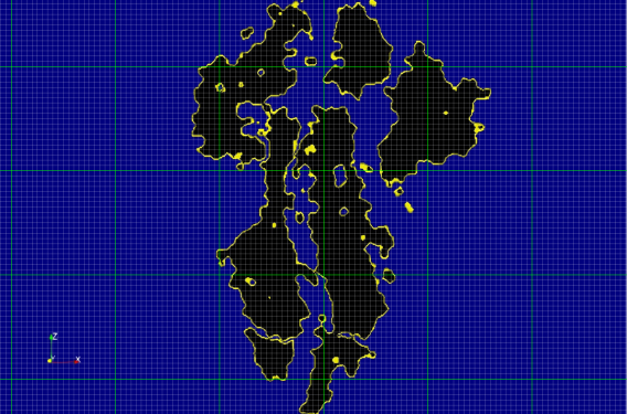  Figure 13: Shows an example grid for a slice of the volumetric image of the Van der Waals surface of the COVID-19 spike glycoprotein (6vxx). The grey grid represents the scalar field whereas the green grid represents possible partitioning of the grid for multithreading. Finer or coarser partitioning may be used depending on the degree of parallelism.
• 
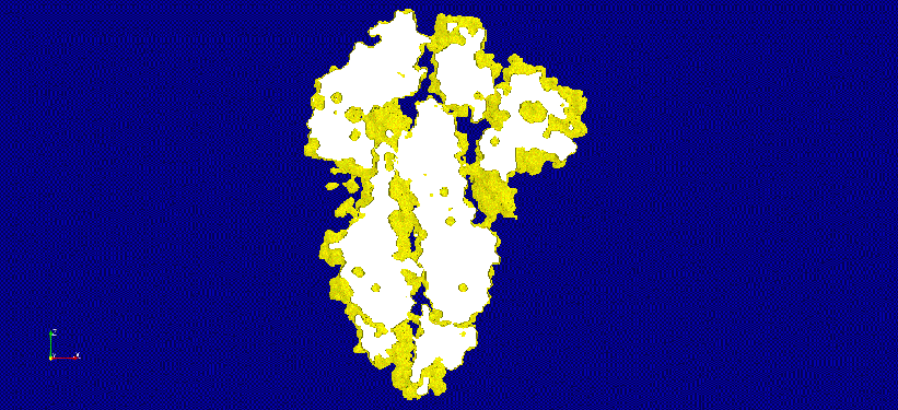  Figure 14: An animation of a thicker slice of the volumetric image of the Van der Waals surface of the COVID-19 spike glycoprotein (6vxx). Potential cavities and voids are clearly visible.

Challenges

There are several challenges that need to be addressed if we are to have a good parallel solution for detecting protein cavities.

1. Expensive Pre-Processing

The parallel methods involving the Van der Waals surface, especially the one with the image input have expensive pre-processing. For large molecules, getting this surface can be slow because existing implementations are sequential and written in Python. We need to come up with a way to quickly generate this surface and its image representation. This pre-processing does not have to be done if we operated on the point cloud using method 2 described previously, leading to a major speedup in overall performance.

Figure 15: The Van der Waals surface of the COVID-19 spike glycoprotein (6vxx).

2. Massive Parallelism (Stretch Goal)

The solution we will implement may need to support massive parallelism, ideally using MPI. The reason for this is that molecular dynamics simulations can potentially involve a massive number of atoms. If we consider the 200 million coronavirus model, then a simulation containing 5000 frames, would involve a total of 1 trillion atoms. If we are to detect the cavities in every frame in real-time, a massively parallel solution is necessary. There is no doubt about why 250,000 CPU cores were required for the COVID-19 simulation.

• 
  Figure 16: An animation produced by a molecular dynamics simulation.
• 
  Figure 17: An animation produced by the COVID-19 molecular dynamics simulation.

Candidate Method: Protein Cavity Identification using Triangulation, unsigned Distance, and Clustering (PCITDC)

The PCITDC method employs Delaunay triangulation to generate a coarse and fine surface of a protein (the fine surface is enclosed within the coarse surface). Then, the unsigned distance of the fine surface from the coarse surface is computed. This is done by iterating through every vertex (atom) in the fine surface and computing its distance from the closest point on the coarse surface. Finally, three-level clustering is employed to cluster atoms based on their distance values.

The algorithm contains the following high-level steps:

(Spiros) Compute Course and Fine surfaces

1. Inaccurate and Accurate Surface Candidates
   1. (Weighted) Delaunay/Voronoi Based:
      1. (Inaccurate) Convex hull (CH) [TODO]
         1. Advantages:
            1. It's easy to calculate
         2. Disadvantages:
            1. The depth values need to be scaled properly in the Unsigned Distance step.
         3. Note: Shared memory parallelism can be employed [TODO]
      2. (Inaccurate and Accurate) Alpha-Shape Surface (AS): [DONE]
         1. Computed using:
            1. Delaunay Triangulation
            2. Removing all tetrahedra of a DT that their circumradius is less than a.
         2. Advantages:
            1. Has a direct relation to the molecule
            2. Has few points -> fast computations further in the pipeline
         3. Disadvantages:
            1. The surface does not help with identifying channels
            2. a needs fine-tuning [TODO]
            3. Many disconnected sub-complexes may be created
         4. Note: parallelism can be employed [TODO]
      3. (Inaccurate and Accurate) Mole Surface (MS): [DONE]
         1. Computed using:
            1. Delaunay Triangulation
            2. First, we remove the boundary tetrahedra. Then we remove all the neighbors of the removed tetrahedra, that none of their vertices satisfy the formula, circumradius < probe-radius + atomRadius. We do that in a BFS fashion till there is no tetrahedron to be removed. This method is similar to AS.
         2. Can be improved by:
            1. Removing slivers using scaled volume, as it was done in PODM3D [TODO]
            2. Not removing elements that incldued at least 3 atomic bond edges [DONE]
            3. Not removing elements that will result in an element have no neighbors [ELIMINATED]
            4. Not removing elements that result in losing vertex of the boundary [ELIMINATED]
         3. Advantages:
            1. Has a direct relation to the molecule
            2. Has few points -> fast computations further in the pipeline
         4. Disadvantages:
            1. The surface does not help with identifying channels
               1. but we can learn from MOLE [TODO]
            2. Probe radius needs fine-tuning [TODO]
         5. Note: parallelism needs to be explored [TODO]
      4. Delaunay Triangulation is performed using Dynamic Parallel Delaunay Triangulation (PDT) [DONE]
         1. Can be improved by:
            1. Implementing a weighted Delaunay Triangulation based on atomic radius [TODO]
         2. Note: Shared memory parallelism can be employed [TODO]
   2. Space Filling Surfaces
      1. (Accurate) Van der Waals surface (WDW) [Done]
         1. Computed using:
            1. Chimera, Programmed in Python (Open-Source) [DONE]
            2. EDT Surf, Programmed in C++ (Open-Source) [TODO]
            3. Chemkit. Programmed in C++ (Open-Source) [TODO]
         2. Advantages:
            1. We can extract all cavities using it
         3. Disadvantages:
            1. Does not have a direct relation to the molecule
            2. Has many points -> slow computations further in the pipeline
         4. Can be improved by:
            1. Clustering decimation which essentially reduces the number of vertices/faces which results in having a reasonable small surface which is a good representation of the molecular surface. [TODO]
            2. Converting it to image and creating a course surface using PODM3D [TODO]
         5. Note: parallelism needs to be explored [TODO]
2. Possible Combinations:
   1. Inaccurate = MS and Accurate = WDW [Done]
      1. Advantages:
         1. Accurate depth evaluation:
      2. Disadvantages:
         1. slow computations further in the pipeline:
   2. Inaccurate = MS and Accurate = MS [Done]
      1. Advantages:
         1. fast computations further in the pipeline:
      2. Disadvantages:
         1. Channels may not be captured
         2. Not as accurate as option (1)
   3. Inaccurate = CH and Accurate = WDW [TODO]
   4. Inaccurate = CH and Accurate = MS [TODO]

(Angelos/Spiros) Compute unsigned distance of the accurate from the inaccurate surface

1. Algorithm:
   1. We iterate through every vertex (atom) in the accurate surface and compute its distance from the closest point on the inaccurate surface. This distance indicates the depth of a specific vertex. We apply Logarithmic scaling.
2. Computed using:
   1. (Angelos) Using vtkStaticCellLocator (octree) [DONE]
      1. Note: Shared memory parallelism can be used [TODO]
   2. (Angelos/Spiros) Using vtkSignedDistance (signed distance) [TODO]
   3. (Spiros) Using path tracing in Delaunay triangulation [TODO]
      1. Algorithmic idea
         1. Find the central cell of the triangulation and then traverse cells using visibility walk and jump and walk techniques in order to minimize the distance with the given point.
         2. Once you reach the boundary, you will have a set of possible cells which include the minimum point, and afterward, you compute it.
      2. Note: Shared memory parallelism can be possibly employed [TODO]

(Angelos/Spiros) Compute atom clusters based on unsigned distance values:

1. (Angelos) A modified version of DBSCAN that finds neighbors based on not only their density but also their unsigned distance values.
   1. Variations:
      1. (Anglelos) One-level clustering [DONE]
      2. (Anglelos) Multi-level clustering to capture all the types of cavities
         1. E.g. Three-level clustering. The first level consists of large surface cavities. The second level consists of small surface cavities. The third level consists of deep cavities (i.e. channels). [DONE]
   2. Modifications:
      1. Implementation-wise:
         1. (Spiros) Use mean cluster-distance value instead of origin first point distance value. [DONE]
      2. Parameters Tuning:
         1. (Spiros) Utilize min/mean/max atom-radius & min/mean/max bondLength to define eps / search-radius [TODO]
         2. (Spiros) Utilize Distibution statistics of distances to define minimum points per cluster. [TODO]
         3. (Angelos) Identify distance areas, e.g. (0-40), where cavities do not exist. [TODO]
   3. Note: parallelism can be employed, see A Fast Parallel Clustering Algorithm for Large Spatial Databases PDBSCAN [TODO]
2. (Angelos/Spiros) A Novel Spatial Clustering Algorithm Based on Delaunay Triangulation [TODO]
   1. Note: parallelism can be explored [TODO]
3. (Angelos) OPTICS: ordering points to identify the clustering structure [TODO]

(Angelos) Classify clusters based on the type of cavity they are:

1. Algorithms:
   1. Unsigned distance based classification using mean distance cluster value [TODO]
      1. Note: Shared memory parallelism can be used [TODO]
   2. Analyze the shape of clusters to identify what type of cavity they are. [TODO]
      1. This can potentially be done using machine learning.
      2. Note: Shared memory parallelism can be used [TODO]

Output:

1. Labeled fine surface [DONE]
2. Labeled protein [TODO]
   1. Note: a Paraview plugin may be developed for visualization purposes.

PCITDC vs MOLE

Feature	PCITDC	MOLE
Detect Surface Cavities	YES (more)	YES (less)
Detect Interior Cavities	YES	YES
Visualize Exact Channel Shape	NO	YES
Works on Very Large Molecules	YES	NO (very slow)
Works on Multi-Model Files	YES	NO
Parallelization	YES	NO
Relative Performance	VERY FAST	SLOW
Intuitive Visualization	YES	YES
False Positives	YES (more)	YES (less)
Quantify Major Structural Features	YES	NO

Resources

• ParaView vertex colors

Resources

Software

• UCSF ChimeraX: Next-generation molecular visualization program from the Resource for Biocomputing, Visualization, and Informatics (RBVI).
• VMD: Molecular visualization program for displaying, animating, and analyzing large biomolecular systems using 3D graphics and built-in scripting. Used in conjunction with NAMD for visualizing molecular dynamics simulations.
• NAMD: Parallel molecular dynamics code designed for high-performance simulation of large biomolecular systems. Scales to hundreds of cores for typical simulations and beyond 500,000 cores for the largest simulations.
• MOLE: Universal toolkit for rapid location and characterization of channels and pores in biomacromolecules.
• CAVER: Software tool for the analysis and visualization of tunnels and channels in protein structures.
• RCSB PDB Protein Data Bank: The largest and most popular database of protein structures.

Papers

• Survey: Geometric Protein Cavity Detection Algorithms: Paper surveying the current geometric algorithms for protein cavity detection. This is a great resource for understanding this project.
• MOLE 2.0: Paper describing the MOLE 2.0 protein cavity detection software. Contains a good algorithm that can be used for extracting a good approximation of the surface of a point cloud of atoms.
• MOLE 1.0: Paper describing the MOLE 1.0 algorithm.
• MolAxis: Paper describing the MolAxis protein cavity detection software.
• CAVER 3.0: Paper describing the CAVER 3.0 protein cavity detection software. This algorithm specializes in identifying tunnels.
• Travel Depth: Paper describing the "travel depth" algorithm for protein cavity visualization.
• GPU Protein Cavity Detection using Ambient Occlusion: Paper describing a GPU-based protein cavity detection algorithm that utilizes Ambient Occlusion.

Organizations/Groups

• University of Illinois at Urbana-Champaign: Theoretical and Computational Biophysics Group: Perhaps the most important group in molecular dynamics. Developers of VMD and NAMD. Ran the simulation for the 200 million atom model of COVID-19.
• Oak Ridge National Laboratory (ORNL): Major national lab with active involvement in drug discovery and design using supercomputers.
• Resource for Biocomputing, Visualization, and Informatics (RBVI): Developers of UCSF Chimera and UCSF ChimeraX.
• IST Austria: Edelsbrunner Group: Important group in algorithms, computational geometry, and computational topology. Involved with protein cavity detection in the past and potentially involved now. The head of the group, Edelsbrunner created alpha shapes.
• Texas Advanced Computing Center: Maintainers of the Frontera supercomputer, the fifth fastest supercomputer in the world (2020). The simulation for the 200 million atom model of COVID-19 was executed on this supercomputer.
• WebChemistry: Developed MOLE and many other software tools related to molecular analysis.

Important Links

• COVID-19 200 million atom NAMD simulation
• ORNL COVID-19 spike drug identification

Proteins

• Large Ribosomal Subunit (98,693 atoms)
• COVID-19 Spike Glycoprotein, Closed State (23,694 atoms)
• COVID-19 Main Protease (5,370 atoms)
• COVID-19 NSP15 Endoribonuclease (24,036 atoms)

References

[1] Simões, T., Lopes, D., Dias, S., Fernandes, F., Pereira, J., Jorge, J., Bajaj, C., & Gomes, A. (2017). Geometric Detection Algorithms for Cavities on Protein Surfaces in Molecular Graphics: A Survey. Computer graphics forum : journal of the European Association for Computer Graphics, 36(8), 643–683. https://doi.org/10.1111/cgf.13158

[2] Yaffe, Fishelovitch, Wolfson, Halperin, & Nussinov. (2008). MolAxis: Efficient and accurate identification of channels in macromolecules. Proteins: Structure, Function, and Bioinformatics, 73(1), 72-86.

[3] Coleman, R. G., & Sharp, K. A. (2006). Travel depth, a new shape descriptor for macromolecules: application to ligand binding. Journal of molecular biology, 362(3), 441–458. https://doi.org/10.1016/j.jmb.2006.07.022