CNF:Mesh Sizing for CNF data
Gradient-based approach for a mesh sizing
Abstract
The data we acquire from Jlab represented evaluations of a “function” on a cube. What it needed is to provide a mesh with a gradation that captures the changes of these values.
Introduction
A similar problem is solved when one refines/adapts a surface mesh with the goal of capturing the curvature of the mesh. In this situation the usual (but not unique) approach is to identify areas of high curvature by styding the deviation of neighboring normals on the surface. If the (normalized) inner product between the normals of two neighboring triangles is close to 1 there is a small angle between them and thus no need for extra refinement . On the other hand as the values of the inner products decreases the angle between the vectors increases and a finer mesh and thus more points are needed to resolve the curvature. The limit and amount of refinement are usually user defined, (see also refine [1] on refining the boundary of the mesh).
Similarly for the case in hand a method based on the local rate of change of values is used.
Method
1. Evaluate the gradient of the image. In the case of the CNF data a simple finite difference stencil is enough, since accuracy is not an issue. ITK has a filter for that already [2].
2. Perform some kind of preprocessing on these data. There are many options here, a literature review of gradient based sizing eg ( [3]) could be usefull. For the results below the transformation is

Intuition:
2.1 “invert” the range by mapping small gradient(small rate of change) to small values and big gradient magnidute (high rate of change) to big values:

2.2 normalize by max to acquire values between 0,1 , in order to remove the notion of size and make it easier to manipulate for the mesh generator program:

2.3 Optionally use a transformation ( in this case square function) to slowdown the size increase (size x^2 < x for x in [0,1])
3. Pass this second image to the mesh generator, scale the value by the diagonal of the bounding box to bring it to input data dimensions and use it to constrain the size of the elements. Optionally support also min and max size as cut-off values.
Notes
- In step 2.2 by nomalizing by max we also loose the “natural” sizing of the data
- In step 2.3 the square is just a convinient transofmation but in some other case another polynomial or even other function, exp,log, tanh could be more appropriate. We can also look in the documentation of AFLR about sizing function in Boundary layer meshes ot any other sizing specific information.
- Step 2.3 is related to the distribution of the data is they are exponential we need something(?) else
Examples
2D
(x^2 +y^2)
-
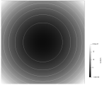 levels sets of two variable function input
-
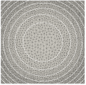 min size =100, tranformation quadratic
-
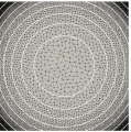 min size =10, tranformation quadratic
-
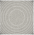 min size =10, tranformation linear


3D
CNF Data looks like it follows exponential distribution,
How do we map exponential distribution properly to element size ?
Is there a more gneric way tha avoid all these complications ?