Difference between revisions of "CNF:Machine Learning"
Pthomadakis (talk | contribs) (→Timeframe) |
|||
| Line 30: | Line 30: | ||
<div class="mw-collapsible mw-collapsed" id="mw-customcollapsible-myToggle1"> | <div class="mw-collapsible mw-collapsed" id="mw-customcollapsible-myToggle1"> | ||
<div class="toccolours mw-collapsible-content"> | <div class="toccolours mw-collapsible-content"> | ||
| + | |||
| + | ===Multilayer Perceptron (80/20 split) === | ||
| + | |||
| + | Accuracy: 0.9531938325991189 | ||
| + | Confusion matrix: | ||
| + | | 933 79| | ||
| + | | 91 2529| | ||
| + | |||
| + | |||
===k-Nearest Neighbors=== | ===k-Nearest Neighbors=== | ||
Revision as of 00:57, 15 September 2019
This is the page for the CNF-Machine Learning project. It will be updated frequently with reports about the progress of the project.
Contents
The Problem
Traditional tracking algorithms are computationally intensive, especially for high luminosity experiments with multi-track final states where all combinations of segments in drift chambers have to be considered for firing best track candidates. At high luminosity the number of random segments (unrelated to the tracks) are increasing and as a result the number of possible combinations also increases, making the whole process longer.
The Goal
Using machine learning one can recognize the patterns that are valid in order to find the correct track faster. The model will be trained on real pre-labeled data and as an outcome, it will be able to label track combinations as valid or not.
The Data
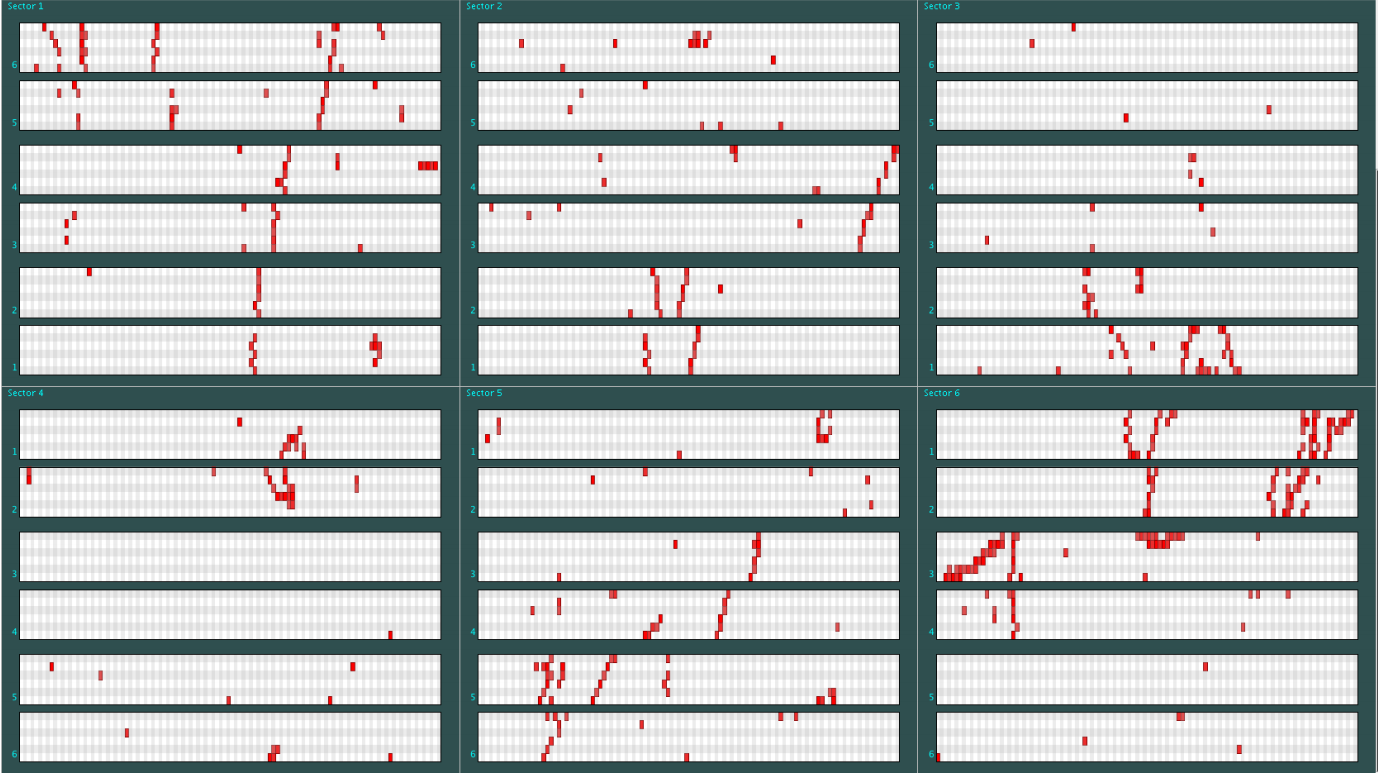
The drift chambers consist of 6 layers, of 6 wires, of 112 sensors each for a total of 4032 sensors (see picture on the right). The data provided let us know whether a sensor has detected a hit or not. Those detections might be part of the trajectory that we want to track or can be irrelevant (noise). The labeled data consist of all the possible combinations that form a track as rows (events) and the state of each sensor (detected something or not) as columns (features). The label provides information on whether a combination produces the valid track or not. An example of the input to be used by the model can be found in [1].
Timeframe
Week 1
Create the pipeline
- Load data in Spark Dataframes
- Split data in training/validation sets
- Experiment with different classification methods
- Tree-based
- SVM
- Train Model
- Validate
- Report accuracy and confusion matrix
Multilayer Perceptron (80/20 split)
Accuracy: 0.9531938325991189 Confusion matrix: | 933 79| | 91 2529|
k-Nearest Neighbors
Accuracy: 0.916
Confusion matrix:
|1861  165|
|448  4790|
Linear SVM
Accuracy: 0.7563325991189427
Confusion matrix:
|409  1617|
|153  5085|
RBF SVM
Accuracy: 0.7210903083700441
Confusion matrix:
|0    2026|
|0    5238|
Gaussian Process
Accuracy: 0.7210903083700441
Confusion matrix:
|0    2026|
|0    5238|
Decision Tree
Accuracy: 0.7231552863436124
Confusion matrix:
|134  1892|
|119  5119|
Random Forest
Accuracy: 0.7210903083700441
Confusion matrix:
|0    2026|
|0    5238|
Neural Net
Accuracy: 0.900330396475771
Confusion matrix:
|1516  510|
|214  5024|
AdaBoost
Accuracy: 0.7221916299559471
Confusion matrix:
|237  1789|
|229  5009|
Naive Bayes
Accuracy: 0.3553138766519824
Confusion matrix:
|1983   43|
|4640  598|
QDA
Accuracy: 0.7581222466960352
Confusion matrix:
|384  1642|
|115  5123|
